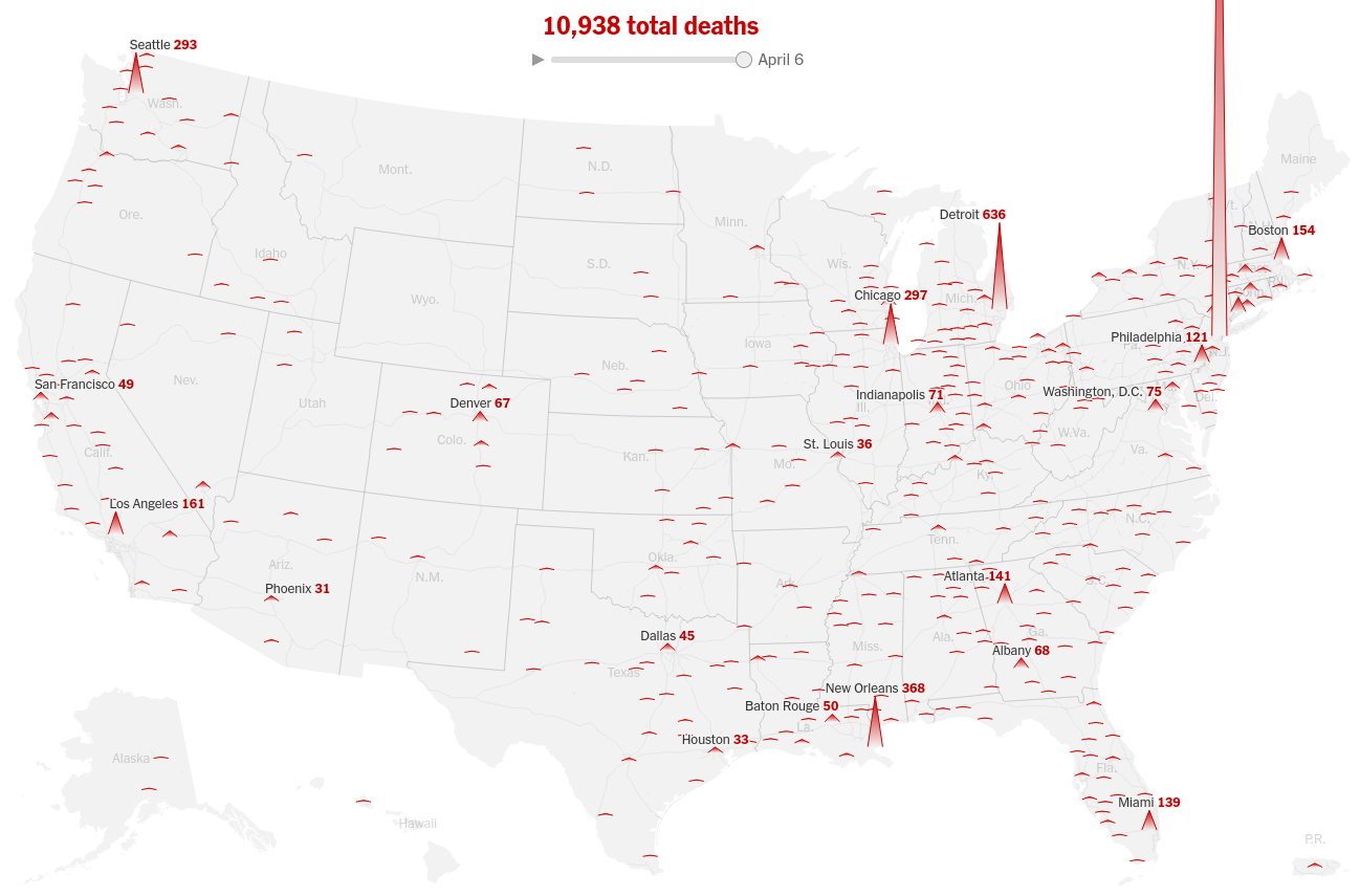
Today we will make a very special graph that looks like the article See How the Coronavirus Death Toll Grew Across the U.S.

deaths spikes

This will require us to use some special techniques using SVG Path elements.

import geopandas as gpd
import altair as alt
import pandas as pd
alt.renderers.set_embed_options(actions=True)
# NYT dataset
county_url = 'https://raw.githubusercontent.com/nytimes/covid-19-data/master/us-counties.csv'
cdf = pd.read_csv(county_url)
cdf.head()
date county state fips cases deaths
0 2020-01-21 Snohomish Washington 53061.0 1 0
1 2020-01-22 Snohomish Washington 53061.0 1 0
2 2020-01-23 Snohomish Washington 53061.0 1 0
3 2020-01-24 Cook Illinois 17031.0 1 0
4 2020-01-24 Snohomish Washington 53061.0 1 0
# Shapefiles from us census
state_shpfile = './shapes/cb_2019_us_state_20m'
county_shpfile = './shapes/cb_2019_us_county_20m'
states = gpd.read_file(state_shpfile)
county = gpd.read_file(county_shpfile)

# Adding longitude and latitude in state data
states['lon'] = states['geometry'].centroid.x
states['lat'] = states['geometry'].centroid.y

# Adding longitude and latitude in county data
county['lon'] = county['geometry'].centroid.x
county['lat'] = county['geometry'].centroid.y

NYT publishes the data for New York City in a different way. So we will add custom FIPS for New York City and Puerto Rico too whose county level information is not present.

cdf.loc[cdf['county'] == 'New York City','fips'] = 1
cdf[cdf['county'] == 'New York City'].head()
date county state fips cases deaths
416 2020-03-01 New York City New York 1.0 1 0
448 2020-03-02 New York City New York 1.0 1 0
482 2020-03-03 New York City New York 1.0 2 0
518 2020-03-04 New York City New York 1.0 2 0
565 2020-03-05 New York City New York 1.0 4 0
cdf.loc[cdf['state'] == 'Puerto Rico', 'fips'] = 2
cdf[cdf['state'] == 'Puerto Rico'].head()
date county state fips cases deaths
1858 2020-03-13 Unknown Puerto Rico 2.0 3 0
2220 2020-03-14 Unknown Puerto Rico 2.0 4 0
2642 2020-03-15 Unknown Puerto Rico 2.0 5 0
3107 2020-03-16 Unknown Puerto Rico 2.0 5 0
3637 2020-03-17 Unknown Puerto Rico 2.0 5 0

Extracting the latest cases and deaths -

aggregate = cdf.groupby('fips', as_index=False).agg({'county': 'first', 'date': 'last', 'state': 'last', 'cases': 'last', 'deaths': 'last'})
aggregate.head()
fips county date state cases deaths
0 1.0 New York City 2020-07-04 New York 221395 22630
1 2.0 Unknown 2020-07-04 Puerto Rico 7787 155
2 1001.0 Autauga 2020-07-04 Alabama 591 13
3 1003.0 Baldwin 2020-07-04 Alabama 863 10
4 1005.0 Barbour 2020-07-04 Alabama 350 2

Combining the 5 boroughs - New York, Kings, Queens, Bronx and Richmond - into one and adding that spatial area in the geodatatrame

#New York City fips = 36005', '36047', '36061', '36081', '36085 which corresponds to New York, Kings, Queens, Bronx and Richmond
spatial_nyc = county[county['GEOID'].isin(['36005', '36047', '36061', '36081', '36085'])]
combined_nyc = spatial_nyc.dissolve(by='STATEFP')
alt.Chart(spatial_nyc).mark_geoshape(stroke='white', strokeWidth=3).encode() | alt.Chart(combined_nyc).mark_geoshape(stroke='white', strokeWidth=3).encode()
agg_nyc_data = spatial_nyc.dissolve(by='STATEFP').reset_index()
agg_nyc_data['GEOID'] = '1'
agg_nyc_data['fips'] = 1
agg_nyc_data['lon'] = agg_nyc_data['geometry'].centroid.x
agg_nyc_data['lat'] = agg_nyc_data['geometry'].centroid.y
county = gpd.GeoDataFrame(pd.concat([county, agg_nyc_data], ignore_index=True))
county['fips'] = county['GEOID']
county['fips'] = county['fips'].astype('int')
county.head()
STATEFP COUNTYFP COUNTYNS AFFGEOID GEOID NAME LSAD ALAND AWATER geometry lon lat fips
0 29 227 00758566 0500000US29227 29227 Worth 06 690564983 493903 POLYGON ((-94.63203 40.57176, -94.53388 40.570... -94.423288 40.479456 29227
1 31 061 00835852 0500000US31061 31061 Franklin 06 1491355860 487899 POLYGON ((-99.17940 40.35068, -98.72683 40.350... -98.952991 40.176363 31061
2 36 013 00974105 0500000US36013 36013 Chautauqua 06 2746047476 1139407865 POLYGON ((-79.76195 42.26986, -79.62748 42.324... -79.366918 42.227692 36013
3 37 181 01008591 0500000US37181 37181 Vance 06 653713542 42178610 POLYGON ((-78.49773 36.51467, -78.45728 36.541... -78.406712 36.368814 37181
4 47 183 01639799 0500000US47183 47183 Weakley 06 1503107848 3707114 POLYGON ((-88.94916 36.41010, -88.81642 36.410... -88.719909 36.298962 47183

We will actually work with Metropolitan Statistical Areas instead of counties, so we need more work to do. We have the MSA Shapefile as well as a dataset that has the counties that combine to form MSAs from the US Census

msa = pd.read_csv('core_msa_list.csv', sep=";")
msa_shp = gpd.read_file('shapes/cb_2019_us_cbsa_500k/cb_2019_us_cbsa_500k.shp')
#msa[msa['CBSA Title'].str.startswith('New York')]
msa.head()
CBSA Code Metropolitan Division Code CSA Code CBSA Title Metropolitan/Micropolitan Statistical Area Metropolitan Division Title CSA Title County/County Equivalent State Name FIPS State Code FIPS County Code Central/Outlying County
0 10100 NaN NaN Aberdeen, SD Micropolitan Statistical Area NaN NaN Brown County South Dakota 46 13 Central
1 10100 NaN NaN Aberdeen, SD Micropolitan Statistical Area NaN NaN Edmunds County South Dakota 46 45 Outlying
2 10140 NaN NaN Aberdeen, WA Micropolitan Statistical Area NaN NaN Grays Harbor County Washington 53 27 Central
3 10180 NaN NaN Abilene, TX Metropolitan Statistical Area NaN NaN Callahan County Texas 48 59 Outlying
4 10180 NaN NaN Abilene, TX Metropolitan Statistical Area NaN NaN Jones County Texas 48 253 Outlying
msa_shp.head()
CSAFP CBSAFP AFFGEOID GEOID NAME LSAD ALAND AWATER geometry
0 425 37620 310M500US37620 37620 Parkersburg-Vienna, WV M1 1551452495 32408833 POLYGON ((-81.75582 39.18052, -81.75575 39.180...
1 None 45980 310M500US45980 45980 Troy, AL M2 1740647520 2336975 POLYGON ((-86.19941 31.80786, -86.19808 31.808...
2 548 49020 310M500US49020 49020 Winchester, VA-WV M1 2752545068 16892497 POLYGON ((-78.97849 39.23900, -78.97626 39.243...
3 142 45180 310M500US45180 45180 Talladega-Sylacauga, AL M2 1908293036 60927931 POLYGON ((-86.50359 33.17598, -86.50313 33.179...
4 None 25060 310M500US25060 25060 Gulfport-Biloxi, MS M1 5739122781 2105780374 MULTIPOLYGON (((-88.50297 30.21523, -88.49176 ...
msa['FIPS State Code'] = msa['FIPS State Code'].astype(str)
msa['FIPS County Code'] = msa['FIPS County Code'].astype(str)
state_fips_max_length = msa['FIPS State Code'].map(len).max()
county_fips_max_length = msa['FIPS County Code'].map(len).max()
msa['FIPS State Code'] = msa['FIPS State Code'].apply(lambda x: '0'*(state_fips_max_length - len(x))+x)
msa['FIPS County Code'] = msa['FIPS County Code'].apply(lambda x: '0'*(county_fips_max_length - len(x))+x)
msa['fips'] = msa['FIPS State Code']+msa['FIPS County Code']
msa['fips'] = msa['fips'].astype(float)

Now we will add a row for New York

nyc_temp = pd.DataFrame({'CBSA Code': 35620,'Metropolitan Division Code': None, 'CSA Code': 408, 'CBSA Title': None,'Metropolitan/Micropolitan Statistical Area': None,	'Metropolitan Division Title': None,'CSA Title': None,'County/County Equivalent': None, 'State Name': 'New York', 'FIPS State Code': 36, 'FIPS County Code': None, 'Central/Outlying County': None, 'fips': 1},index=[0])
msa = pd.concat([msa, nyc_temp], ignore_index=True)
msa
CBSA Code Metropolitan Division Code CSA Code CBSA Title Metropolitan/Micropolitan Statistical Area Metropolitan Division Title CSA Title County/County Equivalent State Name FIPS State Code FIPS County Code Central/Outlying County fips
0 10100 NaN NaN Aberdeen, SD Micropolitan Statistical Area NaN NaN Brown County South Dakota 46 013 Central 46013.0
1 10100 NaN NaN Aberdeen, SD Micropolitan Statistical Area NaN NaN Edmunds County South Dakota 46 045 Outlying 46045.0
2 10140 NaN NaN Aberdeen, WA Micropolitan Statistical Area NaN NaN Grays Harbor County Washington 53 027 Central 53027.0
3 10180 NaN NaN Abilene, TX Metropolitan Statistical Area NaN NaN Callahan County Texas 48 059 Outlying 48059.0
4 10180 NaN NaN Abilene, TX Metropolitan Statistical Area NaN NaN Jones County Texas 48 253 Outlying 48253.0
... ... ... ... ... ... ... ... ... ... ... ... ... ...
1912 49700 NaN 472.0 Yuba City, CA Metropolitan Statistical Area NaN Sacramento-Roseville, CA Yuba County California 06 115 Central 6115.0
1913 49740 NaN NaN Yuma, AZ Metropolitan Statistical Area NaN NaN Yuma County Arizona 04 027 Central 4027.0
1914 49780 NaN 198.0 Zanesville, OH Micropolitan Statistical Area NaN Columbus-Marion-Zanesville, OH Muskingum County Ohio 39 119 Central 39119.0
1915 49820 NaN NaN Zapata, TX Micropolitan Statistical Area NaN NaN Zapata County Texas 48 505 Central 48505.0
1916 35620 None 408.0 None None None None None New York 36 None None 1.0

1917 rows × 13 columns

msa['CBSA Code'] = msa['CBSA Code'].astype(float)
msa[msa['fips'].isin(aggregate['fips']) == False]
CBSA Code Metropolitan Division Code CSA Code CBSA Title Metropolitan/Micropolitan Statistical Area Metropolitan Division Title CSA Title County/County Equivalent State Name FIPS State Code FIPS County Code Central/Outlying County fips
8 10380.0 NaN NaN Aguadilla-Isabela, PR Metropolitan Statistical Area NaN NaN Aguada Municipio Puerto Rico 72 003 Central 72003.0
9 10380.0 NaN NaN Aguadilla-Isabela, PR Metropolitan Statistical Area NaN NaN Aguadilla Municipio Puerto Rico 72 005 Central 72005.0
10 10380.0 NaN NaN Aguadilla-Isabela, PR Metropolitan Statistical Area NaN NaN Añasco Municipio Puerto Rico 72 011 Central 72011.0
11 10380.0 NaN NaN Aguadilla-Isabela, PR Metropolitan Statistical Area NaN NaN Isabela Municipio Puerto Rico 72 071 Central 72071.0
12 10380.0 NaN NaN Aguadilla-Isabela, PR Metropolitan Statistical Area NaN NaN Lares Municipio Puerto Rico 72 081 Central 72081.0
... ... ... ... ... ... ... ... ... ... ... ... ... ...
1591 42180.0 NaN 434.0 Santa Isabel, PR Micropolitan Statistical Area NaN Ponce-Yauco-Coamo, PR Santa Isabel Municipio Puerto Rico 72 133 Central 72133.0
1903 49500.0 NaN 434.0 Yauco, PR Metropolitan Statistical Area NaN Ponce-Yauco-Coamo, PR Guánica Municipio Puerto Rico 72 055 Central 72055.0
1904 49500.0 NaN 434.0 Yauco, PR Metropolitan Statistical Area NaN Ponce-Yauco-Coamo, PR Guayanilla Municipio Puerto Rico 72 059 Central 72059.0
1905 49500.0 NaN 434.0 Yauco, PR Metropolitan Statistical Area NaN Ponce-Yauco-Coamo, PR Peñuelas Municipio Puerto Rico 72 111 Central 72111.0
1906 49500.0 NaN 434.0 Yauco, PR Metropolitan Statistical Area NaN Ponce-Yauco-Coamo, PR Yauco Municipio Puerto Rico 72 153 Central 72153.0

88 rows × 13 columns

# Puerto Rico does not provide data at county level. So we will have to do a similar exercise like NYC for PR and aggregate it statewise. 
# But since in albersUsa projection PR is filtered anyways, we won't be doing that exercise right away. Once I figure out how to use custom projection in the default
# albersUsa projection that is used by Vega-Lite under the hood, we will include Puerto Rico
aggregate[aggregate['state'].str.startswith('Puerto')]
fips county date state cases deaths
1 2.0 Unknown 2020-07-04 Puerto Rico 7787 155
aggregate[aggregate['fips'].isin(msa['fips']) == False]
fips county date state cases deaths
1 2.0 Unknown 2020-07-04 Puerto Rico 7787 155
7 1011.0 Bullock 2020-07-04 Alabama 373 11
8 1013.0 Butler 2020-07-04 Alabama 626 28
11 1019.0 Cherokee 2020-07-04 Alabama 88 7
13 1023.0 Choctaw 2020-07-04 Alabama 196 12
... ... ... ... ... ... ...
3052 56027.0 Niobrara 2020-07-04 Wyoming 2 0
3053 56029.0 Park 2020-07-04 Wyoming 61 0
3054 56031.0 Platte 2020-07-04 Wyoming 4 0
3056 56035.0 Sublette 2020-07-04 Wyoming 6 0
3060 56043.0 Washakie 2020-07-04 Wyoming 38 5

1233 rows × 6 columns

Now we will merge the aggregated data with msa since msa is expanded on fips(CBSA repeats), which is the only unique column.

msa = msa.merge(aggregate, how='inner', on='fips')
msa
CBSA Code Metropolitan Division Code CSA Code CBSA Title Metropolitan/Micropolitan Statistical Area Metropolitan Division Title CSA Title County/County Equivalent State Name FIPS State Code FIPS County Code Central/Outlying County fips county date state cases deaths
0 10100.0 NaN NaN Aberdeen, SD Micropolitan Statistical Area NaN NaN Brown County South Dakota 46 013 Central 46013.0 Brown 2020-07-04 South Dakota 343 2
1 10100.0 NaN NaN Aberdeen, SD Micropolitan Statistical Area NaN NaN Edmunds County South Dakota 46 045 Outlying 46045.0 Edmunds 2020-07-04 South Dakota 8 0
2 10140.0 NaN NaN Aberdeen, WA Micropolitan Statistical Area NaN NaN Grays Harbor County Washington 53 027 Central 53027.0 Grays Harbor 2020-07-04 Washington 26 0
3 10180.0 NaN NaN Abilene, TX Metropolitan Statistical Area NaN NaN Callahan County Texas 48 059 Outlying 48059.0 Callahan 2020-07-04 Texas 19 2
4 10180.0 NaN NaN Abilene, TX Metropolitan Statistical Area NaN NaN Jones County Texas 48 253 Outlying 48253.0 Jones 2020-07-04 Texas 610 0
... ... ... ... ... ... ... ... ... ... ... ... ... ... ... ... ... ... ...
1824 49700.0 NaN 472.0 Yuba City, CA Metropolitan Statistical Area NaN Sacramento-Roseville, CA Yuba County California 06 115 Central 6115.0 Yuba 2020-07-04 California 120 2
1825 49740.0 NaN NaN Yuma, AZ Metropolitan Statistical Area NaN NaN Yuma County Arizona 04 027 Central 4027.0 Yuma 2020-07-04 Arizona 7062 110
1826 49780.0 NaN 198.0 Zanesville, OH Micropolitan Statistical Area NaN Columbus-Marion-Zanesville, OH Muskingum County Ohio 39 119 Central 39119.0 Muskingum 2020-07-04 Ohio 81 1
1827 49820.0 NaN NaN Zapata, TX Micropolitan Statistical Area NaN NaN Zapata County Texas 48 505 Central 48505.0 Zapata 2020-07-04 Texas 56 0
1828 35620.0 None 408.0 None None None None None New York 36 None None 1.0 New York City 2020-07-04 New York 221395 22630

1829 rows × 18 columns

msa.rename(columns={'CBSA Code': 'CBSAFP'}, inplace=True)
msa_shp['CBSAFP'] = msa_shp['CBSAFP'].astype(float)
msa_shp['lon'] = msa_shp['geometry'].centroid.x
msa_shp['lat'] = msa_shp['geometry'].centroid.y

Now we will aggregate the msa data on CBSAFP so that it becomes similar to msa_shp geodataframe

msa_agg = msa.groupby('CBSAFP', as_index=False).agg({'CBSA Title': 'first', 'State Name': 'last', 'date': 'last', 'cases': 'sum', 'deaths': 'sum'})
msa_agg.head()
CBSAFP CBSA Title State Name date cases deaths
0 10100.0 Aberdeen, SD South Dakota 2020-07-04 351 2
1 10140.0 Aberdeen, WA Washington 2020-07-04 26 0
2 10180.0 Abilene, TX Texas 2020-07-04 1209 8
3 10220.0 Ada, OK Oklahoma 2020-07-04 44 2
4 10300.0 Adrian, MI Michigan 2020-07-04 966 10

Now we will merge msa_agg with msa and make the heights column that contains a custom SVG Path string per row, since right now Vega-Lite does not support "scaleY" as an encoding. In Vega, we don't have to do it this way, we can just provide a single svg path for an equilateral triangle and then stretch it(using scaleY) based on "cases" or "deaths".

msa_shp = msa_shp.merge(msa_agg, how='inner', on='CBSAFP')
msa_shp['height'] = msa_shp['deaths'].apply(lambda x: f"M -1.5 0 L0 -{x/50} L1.5 0" if pd.notnull(x) else "M -1.5 0 L0 0 L1.5 0")
msa_shp.head()
CSAFP CBSAFP AFFGEOID GEOID NAME LSAD ALAND AWATER geometry lon lat CBSA Title State Name date cases deaths height
0 425 37620.0 310M500US37620 37620 Parkersburg-Vienna, WV M1 1551452495 32408833 POLYGON ((-81.75582 39.18052, -81.75575 39.180... -81.462789 39.138851 Parkersburg-Vienna, WV West Virginia 2020-07-04 123 2 M -1.5 0 L0 -0.04 L1.5 0
1 None 45980.0 310M500US45980 45980 Troy, AL M2 1740647520 2336975 POLYGON ((-86.19941 31.80786, -86.19808 31.808... -85.940915 31.802723 Troy, AL Alabama 2020-07-04 427 5 M -1.5 0 L0 -0.1 L1.5 0
2 548 49020.0 310M500US49020 49020 Winchester, VA-WV M1 2752545068 16892497 POLYGON ((-78.97849 39.23900, -78.97626 39.243... -78.473885 39.272178 Winchester, VA-WV West Virginia 2020-07-04 892 10 M -1.5 0 L0 -0.2 L1.5 0
3 142 45180.0 310M500US45180 45180 Talladega-Sylacauga, AL M2 1908293036 60927931 POLYGON ((-86.50359 33.17598, -86.50313 33.179... -86.165882 33.380087 Talladega-Sylacauga, AL Alabama 2020-07-04 311 8 M -1.5 0 L0 -0.16 L1.5 0
4 None 25060.0 310M500US25060 25060 Gulfport-Biloxi, MS M1 5739122781 2105780374 MULTIPOLYGON (((-88.50297 30.21523, -88.49176 ... -89.037857 30.556428 Gulfport-Biloxi, MS Mississippi 2020-07-04 1692 40 M -1.5 0 L0 -0.8 L1.5 0
msa_shp.drop(['CSAFP', 'AFFGEOID', 'GEOID', 'LSAD', 'ALAND', 'AWATER'], axis=1, inplace=True)
msa_shp.head()
CBSAFP NAME geometry lon lat CBSA Title State Name date cases deaths height
0 37620.0 Parkersburg-Vienna, WV POLYGON ((-81.75582 39.18052, -81.75575 39.180... -81.462789 39.138851 Parkersburg-Vienna, WV West Virginia 2020-07-04 123 2 M -1.5 0 L0 -0.04 L1.5 0
1 45980.0 Troy, AL POLYGON ((-86.19941 31.80786, -86.19808 31.808... -85.940915 31.802723 Troy, AL Alabama 2020-07-04 427 5 M -1.5 0 L0 -0.1 L1.5 0
2 49020.0 Winchester, VA-WV POLYGON ((-78.97849 39.23900, -78.97626 39.243... -78.473885 39.272178 Winchester, VA-WV West Virginia 2020-07-04 892 10 M -1.5 0 L0 -0.2 L1.5 0
3 45180.0 Talladega-Sylacauga, AL POLYGON ((-86.50359 33.17598, -86.50313 33.179... -86.165882 33.380087 Talladega-Sylacauga, AL Alabama 2020-07-04 311 8 M -1.5 0 L0 -0.16 L1.5 0
4 25060.0 Gulfport-Biloxi, MS MULTIPOLYGON (((-88.50297 30.21523, -88.49176 ... -89.037857 30.556428 Gulfport-Biloxi, MS Mississippi 2020-07-04 1692 40 M -1.5 0 L0 -0.8 L1.5 0

Let's finally plot this graph of deaths till now -

spikes = alt.Chart(msa_shp).transform_filter(alt.datum.deaths>0).mark_point(
    fillOpacity=1, 
    fill=alt.Gradient(
        gradient="linear",
        stops=[alt.GradientStop(color='white', offset=0), alt.GradientStop(color='red', offset=0.5)],
        x1=1,
        x2=1,
        y1=1,
        y2=0 
    ), 
    #dx=10, 
    #dy=-30, 
    strokeOpacity=1, 
    strokeWidth=1,
    stroke='red'
).encode(
    latitude="lat:Q",
    longitude="lon:Q",
    shape=alt.Shape("height:N", scale=None),
    #tooltip=['CBSA Title:N', 'deaths:Q'],
    #color = alt.condition(selection, alt.value('black'), alt.value('red'))
).project(
    type='albersUsa'
).properties(
    width=1200,
    height=800
)

state = alt.Chart(states).mark_geoshape(fill='#ededed', stroke='white').encode(
).project(
    type='albersUsa'
)

(state+spikes).configure_view(strokeWidth=0)

Now we will study only last week's average cases per day to see where the indections are on the rise

#msa_shp['height_cases'] = msa_shp['cases'].apply(lambda x: f"M -1.5 0 L0 -{x/1000} L1.5 0" if pd.notnull(x) else "M -1.5 0 L0 0 L1.5 0")
cdf['cases_per_day'] = cdf.groupby("fips")['cases'].diff()
last_week_cases_avg = cdf.groupby("fips")["cases_per_day"].apply(lambda x: x.iloc[-7:].mean())
last_week_cases_avg = last_week_cases_avg.reset_index()
last_week_cases_avg.columns = ['fips', 'avg_cases_last_week']
last_week_cases_avg.head()
fips avg_cases_last_week
0 1.0 319.714286
1 2.0 103.000000
2 1001.0 13.285714
3 1003.0 44.000000
4 1005.0 4.714286
avg_last_week_cases = cdf.groupby("fips").agg({'county': 'first', 'cases_per_day': 'last', 'date': 'last', 'state': 'last', 'cases': 'last', 'deaths': 'last'})
avg_last_week_cases = avg_last_week_cases.merge(last_week_cases_avg, how='inner', on='fips')
avg_last_week_cases.head()
fips county cases_per_day date state cases deaths avg_cases_last_week
0 1.0 New York City 367.0 2020-07-04 New York 221395 22630 319.714286
1 2.0 Unknown 104.0 2020-07-04 Puerto Rico 7787 155 103.000000
2 1001.0 Autauga 23.0 2020-07-04 Alabama 591 13 13.285714
3 1003.0 Baldwin 18.0 2020-07-04 Alabama 863 10 44.000000
4 1005.0 Barbour 2.0 2020-07-04 Alabama 350 2 4.714286
msa_agg_lastweek = msa.merge(avg_last_week_cases, how='inner', on='fips')
msa_agg_lastweek.head()
CBSAFP Metropolitan Division Code CSA Code CBSA Title Metropolitan/Micropolitan Statistical Area Metropolitan Division Title CSA Title County/County Equivalent State Name FIPS State Code ... state_x cases_x deaths_x county_y cases_per_day date_y state_y cases_y deaths_y avg_cases_last_week
0 10100.0 NaN NaN Aberdeen, SD Micropolitan Statistical Area NaN NaN Brown County South Dakota 46 ... South Dakota 343 2 Brown -1.0 2020-07-04 South Dakota 343 2 0.571429
1 10100.0 NaN NaN Aberdeen, SD Micropolitan Statistical Area NaN NaN Edmunds County South Dakota 46 ... South Dakota 8 0 Edmunds 1.0 2020-07-04 South Dakota 8 0 0.142857
2 10140.0 NaN NaN Aberdeen, WA Micropolitan Statistical Area NaN NaN Grays Harbor County Washington 53 ... Washington 26 0 Grays Harbor 0.0 2020-07-04 Washington 26 0 0.142857
3 10180.0 NaN NaN Abilene, TX Metropolitan Statistical Area NaN NaN Callahan County Texas 48 ... Texas 19 2 Callahan 1.0 2020-07-04 Texas 19 2 0.428571
4 10180.0 NaN NaN Abilene, TX Metropolitan Statistical Area NaN NaN Jones County Texas 48 ... Texas 610 0 Jones 0.0 2020-07-04 Texas 610 0 0.428571

5 rows × 25 columns

# Average of multiple series is same as sum of their averages so 'avg_cases_last_week': 'sum' works well
msa_agg_lastweek = msa_agg_lastweek.groupby('CBSAFP', as_index=False).agg({'CBSA Title': 'first', 'State Name': 'last', 'avg_cases_last_week': 'sum'})
msa_agg_lastweek.head()
CBSAFP CBSA Title State Name avg_cases_last_week
0 10100.0 Aberdeen, SD South Dakota 0.714286
1 10140.0 Aberdeen, WA Washington 0.142857
2 10180.0 Abilene, TX Texas 21.857143
3 10220.0 Ada, OK Oklahoma 1.285714
4 10300.0 Adrian, MI Michigan 4.000000
msa_shp = msa_shp.merge(msa_agg_lastweek, how='inner', on='CBSAFP')
msa_shp.head()
CBSAFP NAME geometry lon lat CBSA Title_x State Name_x date cases deaths height CBSA Title_y State Name_y avg_cases_last_week
0 37620.0 Parkersburg-Vienna, WV POLYGON ((-81.75582 39.18052, -81.75575 39.180... -81.462789 39.138851 Parkersburg-Vienna, WV West Virginia 2020-07-04 123 2 M -1.5 0 L0 -0.04 L1.5 0 Parkersburg-Vienna, WV West Virginia 6.428571
1 45980.0 Troy, AL POLYGON ((-86.19941 31.80786, -86.19808 31.808... -85.940915 31.802723 Troy, AL Alabama 2020-07-04 427 5 M -1.5 0 L0 -0.1 L1.5 0 Troy, AL Alabama 4.714286
2 49020.0 Winchester, VA-WV POLYGON ((-78.97849 39.23900, -78.97626 39.243... -78.473885 39.272178 Winchester, VA-WV West Virginia 2020-07-04 892 10 M -1.5 0 L0 -0.2 L1.5 0 Winchester, VA-WV West Virginia 9.000000
3 45180.0 Talladega-Sylacauga, AL POLYGON ((-86.50359 33.17598, -86.50313 33.179... -86.165882 33.380087 Talladega-Sylacauga, AL Alabama 2020-07-04 311 8 M -1.5 0 L0 -0.16 L1.5 0 Talladega-Sylacauga, AL Alabama 11.857143
4 25060.0 Gulfport-Biloxi, MS MULTIPOLYGON (((-88.50297 30.21523, -88.49176 ... -89.037857 30.556428 Gulfport-Biloxi, MS Mississippi 2020-07-04 1692 40 M -1.5 0 L0 -0.8 L1.5 0 Gulfport-Biloxi, MS Mississippi 60.000000

Adding a new column called height_last_week_avg_cases that has the custom SVG paths like we did earlier -

msa_shp['height_last_week_avg_cases'] = msa_shp['avg_cases_last_week'].apply(lambda x: f"M -1.5 0 L0 -{x/10} L1.5 0" if pd.notnull(x) else "M -1.5 0 L0 0 L1.5 0")
spikes = alt.Chart(msa_shp).mark_point(
    fillOpacity=1, 
    fill=alt.Gradient(
        gradient="linear",
        stops=[alt.GradientStop(color='white', offset=0), alt.GradientStop(color='red', offset=0.5)],
        x1=1,
        x2=1,
        y1=1,
        y2=0 
    ), 
    #dx=10, 
    #dy=-30,
    stroke='red',
    strokeOpacity=1, 
    strokeWidth=1
).encode(
    latitude="lat:Q",
    longitude="lon:Q",
    shape=alt.Shape("height_last_week_avg_cases:N", scale=None),
    tooltip=['NAME:N', 'avg_cases_last_week:Q']
).project(
    type='albersUsa'
).properties(
    width=1200,
    height=800
)

state = alt.Chart(states).mark_geoshape(fill='#ededed', stroke='white').encode(
).project(
    type='albersUsa'
)

(state+spikes).configure_view(strokeWidth=0)

It's clear that now the cases are increasing much rapidly in the South especially in the states of - Texas, California, Florida and Arizona

There you have it!