Decrease in GDP of USA
Bar chart created as faceted chart

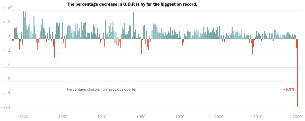
Tis post will show you how to make the GDP chart in the article by titled Big Tech Earnings Surge as Economy Slumps
Nothing that it's a percent change from previous quarter data, we will extract the data for this chart as follows from Bureau of Economic Analysis -
- Go here - https://apps.bea.gov/iTable/index_nipa.cfm
- Click on "Begin using this data"
- Click on Section 1
- Click on Table 1.1.1 - Percent Change From Preceding Period in Real Gross Domestic Product - Annualized
- Click on Modify
- Select on all years
- Repeat the steps for Table 1.1.3 - Real Gross Domestic Product, Quantity Indexes
Now you know that GDP is reported in a rather peculiar way - annulazied GDP. It mean's they report values of GDP such that if the current state of affairs continue then what would happen by the end of the year
The formula for annunalizing is -
$ g_{m} = \left[ \left( \frac{X_{m}}{X_{m-1}} \right)^n -1 \right]\cdot100 $
where n is 4 for quarterly available data and 12 for monthly data
import pandas as pd
import altair as alt
from functools import wraps
import datetime as dt

alt.renderers.set_embed_options(actions=False)

def log_step(func):
    @wraps(func)
    def wrapper(*args, **kwargs):
        """timing or logging etc"""
        start = dt.datetime.now()
        output = func(*args, **kwargs)
        end = dt.datetime.now()
        print(f"After function {func.__name__} ran, shape of dataframe is - {output.shape}, execution time is - {end-start}")
        return output
    return wrapper

@log_step
def read_transpose_gdp_data(path, if_uri):
    if if_uri:
        pass
    else:
        cols = pd.read_csv(path, skiprows=4, header=None, nrows=1)
        us_gdp = pd.read_csv(path, skiprows=4, header=None, usecols=[i for i in cols if i != 0])
        us_gdp = us_gdp.T
        us_gdp.iloc[0,0] = 'year'
        us_gdp.iloc[0,1] = 'quarter'
        us_gdp.columns = us_gdp.iloc[0]
        us_gdp = us_gdp[1:]
        return us_gdp

@log_step
def clean_gdp_data(df):
    df.columns = [x.strip() for x in df.columns]
    #df.columns = [x.strip() if type(x) != float else x for x in list(df.columns)]
    df['Gross domestic product'] = df['Gross domestic product'].astype(float)
    df['year'] = df['year'].astype(int)
    df = df.reset_index(drop=True)
    #df.rename(columns={'Gross domestic product': 'gdp'}, inplace=True)
    #df['year'] = pd.to_datetime(df['year'], format="%Y")
    df.drop(df.columns[3:], inplace=True, axis=1)
    return df

@log_step
def rename_cols(df, col_dict):
    df.rename(columns=col_dict, inplace=True)
    return df

@log_step
def assign_columns(df):
    df = df.assign(non_annualized_gdp = df['real_gdp'].diff()/df['real_gdp'].shift(1)*100)
    return df

@log_step
def reshape_concat_column(df, col):
    df = df[1:].reset_index()
    df = df.assign(annualized_gdp = col)
    return df

def year_as_time(df):
    df['year'] = pd.to_datetime(df['year'], format="%Y")
    return df
ann_gdp = (read_transpose_gdp_data(path='usa_gdp.csv', if_uri=False)
          .pipe(clean_gdp_data)
          .pipe(rename_cols, col_dict={'Gross domestic product': 'ann_gdp'})
         )

ann_gdp.head()
When we plot this we will find that it looks very much like the graph in the article. We just have to play around the facet spacings to make it look continuous like a single bar chart instead of a faceted chart
alt.Chart(ann_gdp).mark_bar(width=5).encode(
    x=alt.X('quarter:O', title=None, axis=alt.Axis(labels=False, ticks=False)),
    y='ann_gdp:Q',
    facet=alt.Facet('year:O', bounds='flush', spacing={'column':0}, header=alt.Header(labels=False, title=None)),
    #detail='quarter:N',
    color=alt.condition(alt.datum.ann_gdp > 0, alt.value('green'), alt.value('red'))
).configure_axis(grid=False).configure_view(strokeWidth=1, step=5)
The chart you see above is the annualized GDP which suggests that the US economy will shrink by a third if things stay exactly like the way they are now. Which is certainly not representative of current times. Fortunately the BEA also provides the Real GDP as Quantity Index units. If you apply the formaula to that data you get the data above i.e Table 1.1.1. Real GDP is a transformed version of nominal GDP Let's chart Table
Nominal GDP is reported as billions or trillions of dollars
re_gdp = (read_transpose_gdp_data(path='us_gdp.csv', if_uri=False)
           .pipe(clean_gdp_data)
           .pipe(rename_cols, col_dict={'Gross domestic product': 'real_gdp'}))

re_gdp.head()
Plotting this we will see how GDP has increased over the years -
alt.Chart(re_gdp).mark_bar(width=3.25).encode(
    x=alt.X('quarter:O', title=None, axis=alt.Axis(labels=False, ticks=False)),
    y='real_gdp:Q',
    column = alt.Facet('year:O', spacing=0, header=alt.Header(labels=False, title=None))

).configure_view(strokeWidth=0, step=4)
Let's calculate non-annualized gdp from the real gdp -
usa_gdp = re_gdp.pipe(assign_columns)
usa_gdp.head()
Highlighting the quarters where we had negative growth compared to previous quarter (using non-annualized gdp) -
alt.Chart(usa_gdp).mark_bar(width=3.25).encode(
    x=alt.X('quarter:O', title=None, axis=alt.Axis(labels=False, ticks=False)),
    y='real_gdp:Q',
    column=alt.Facet('year:O', spacing=0, header=alt.Header(labels=False, title=None)),
    #detail='quarter:N',
    color=alt.condition(alt.datum.non_annualized_gdp > 0, alt.value('#76a4a5'), alt.value('#d0573a'))
).configure_axis(grid=True).configure_view(strokeWidth=0, step=4)
Finally let's plot the non-annualized GDP. We will see that it's no longer close to -30 but to -10, just like the chart in the article.
alt.Chart(usa_gdp).mark_bar(width=3.25).encode(
    x=alt.X('quarter:O', title=None, axis=alt.Axis(labels=False, ticks=False)),
    y='non_annualized_gdp:Q',
    column=alt.Facet('year:O', spacing=0, header=alt.Header(labels=False, title=None)),
    #detail='quarter:N',
    color=alt.condition(alt.datum.non_annualized_gdp > 0, alt.value('#76a4a5'), alt.value('#d0573a'))
).configure_axis(grid=False).configure_view(strokeWidth=0, step=4)
Let's add annualized gdp data to real and non-annualized gdp data to that we may plot them together for a bigger picture
usa_gdp = (usa_gdp
          .pipe(reshape_concat_column, ann_gdp['ann_gdp']) # because Annualized GDP and Real GDP have different shapes
          .pipe(year_as_time))

usa_gdp.head()
To see the contrast b/w the two to understand how misleading annualized gdp can be we will layer them on top of each other -
a = alt.Chart().mark_bar(width=3.25).encode(
    x=alt.X('quarter:O', title=None, axis=alt.Axis(labels=False, domain=False, ticks=False)),
    y='non_annualized_gdp:Q',
    #column=alt.Facet('year:O', spacing=0, header=alt.Header(labels=False, title=None)),
    #detail='quarter:N',
    color=alt.condition(alt.datum.non_annualized_gdp > 0, alt.value('blue'), alt.value('maroon')),
    #text = 'num:Q'
)

b = alt.Chart().mark_bar(width=3.25).encode(
    x=alt.X('quarter:O', title=None, axis=alt.Axis(labels=False, ticks=False)),
    y='annualized_gdp:Q',
    #column=alt.Facet('year:O', spacing=0, header=alt.Header(labels=False, title=None)),
    #detail='quarter:N',
    color=alt.condition(alt.datum.annualized_gdp > 0, alt.value('orange'), alt.value('violet')),
)

n_ann_gdp = alt.Chart().transform_filter({'field': 'year', 'oneOf': [2008, 2020], 'timeUnit': 'year'}).mark_text(color='maroon', dx=-12, dy=7, fontSize=12).encode(
    x=alt.X('quarter:O', title=None, aggregate={'argmin': 'non_annualized_gdp'}),# axis=alt.Axis(labels=False, domain=False, ticks=False)),
    y='min(non_annualized_gdp):Q',
    text=alt.Text('min(non_annualized_gdp):Q', format='.2', )
    #x=alt.X('quarter', aggregate={'argmin': 'non_annualized_gdp'})
)

ann_gdp = alt.Chart().transform_filter(alt.FieldOneOfPredicate(field='year', oneOf=[2008, 2020], timeUnit='year')).mark_text(color='violet', dx=-12, dy=0, fontSize=12).encode(
    x=alt.X('quarter:O', title=None, aggregate={'argmin': 'annualized_gdp'}),# axis=alt.Axis(labels=False, domain=False, ticks=False)),
    y=alt.Y('min(annualized_gdp):Q', title='Annualized GDP,  Real GDP'),
    text=alt.Text('min(annualized_gdp):Q', format='.2', )
    #x=alt.X('quarter', aggregate={'argmin': 'non_annualized_gdp'})
)

alt.layer(b, a, n_ann_gdp, ann_gdp, data=usa_gdp).facet(
    column=alt.Facet('year:T', header=alt.Header(labels=True, labelColor='grey', labelOrient='bottom', format="%y", formatType='time', title=None)),
    spacing=0,
    bounds='flush'
).configure_axis(domain=False,
                 labelColor='grey',
                 tickColor='lightgrey',
                 domainColor='lightgrey',
                 titleColor='grey'
                ).configure_view(strokeWidth=0, step=4).configure_axisY(grid=True,)
We can see clearly that the damage to the economy is greater than the 2008 recession